Machine learning is a branch of artificial intelligence that allows systems to learn from data and make predictions or decisions without being explicitly programmed. It is a method of teaching computers to learn from data, identify patterns and make decisions with minimal human intervention.

The steps in a typical machine learning project include:

Project Idea: Predicting the prices of used cars based on their mileage and age.

Step 1: Collect and prepare the data. You can use a publicly available dataset, such as the “Automobile Dataset” from the UCI Machine Learning Repository or you can scrape the data from a website such as Craigslist or Carfax. Once you have the data, you will need to clean it and remove any missing or invalid values.

You can load the Boston Housing dataset using the scikit-learn library.

from sklearn.datasets import load_boston

# Load the Boston Housing dataset
boston = load_boston()

# Split the data into input (X) and output (y)
X = boston.data
y = boston.target

Step 2: Exploratory Data Analysis (EDA). You will need to investigate the data, create visualizations and compute statistics to understand the distribution and relationship between the features and the target variable (car price).

You can use the pandas and seaborn library to create visualizations and compute statistics to understand the distribution and relationship between the features and the target variable (house prices).

import pandas as pd
import seaborn as sns

# Create a DataFrame from the data
df = pd.DataFrame(boston.data, columns=boston.feature_names)
df['PRICE'] = boston.target

# Create a pairplot to visualize the relationship between the features
sns.pairplot(df, x_vars=boston.feature_names, y_vars='PRICE')

# Compute basic statistics for the data
print(df.describe())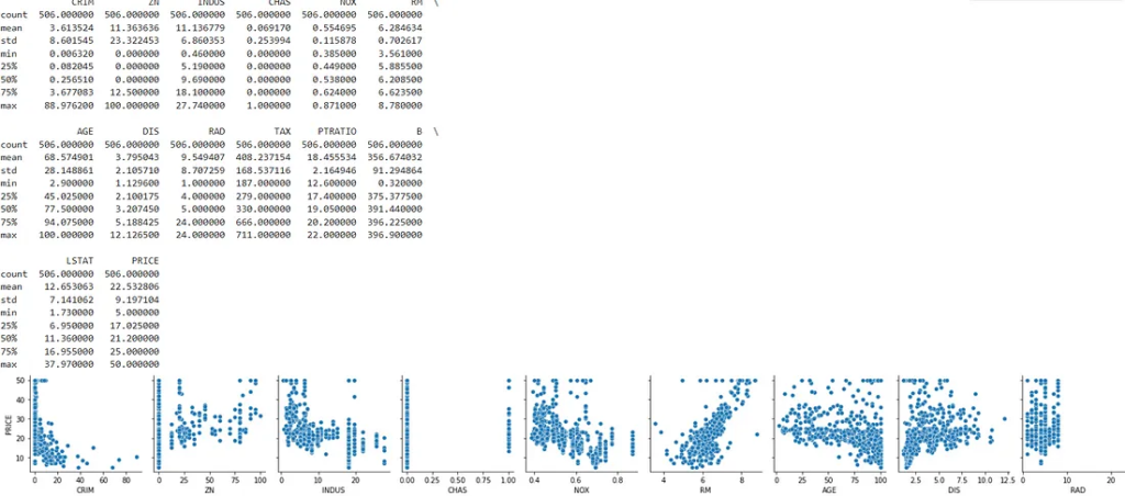

Step 3: Feature Engineering. Based on the findings from the EDA, you will need to engineer new features and/or transform existing ones to improve the performance of the model. For example, you could create a new feature that represents the ratio of rooms to the total area of the house or a feature that represents the age of the house.

# Create a new feature that represents the ratio of rooms to the total area of the house
df['ROOM_RATIO'] = df['RM'] / df['LSTAT']

# Create a new feature that represents the age of the house
df['AGE'] = df['DIS'] * df['TAX']

Step 4: Split the data into training and test sets.

You can use the scikit-learn library to train a linear regression model on the training data.

from sklearn.model_selection import train_test_split

# Split the data into training and test sets
X_train, X_test, y_train, y_test = train_test_split(X, y, test_size=0.2)

Step 5: Define, compile and train the model. You can use a library such as scikit-learn or Keras to train a linear regression model on the training data.

You can use metrics such as mean squared error or R-squared to evaluate the performance of the model.

from sklearn.linear_model import LinearRegression

# Create an instance of the linear regression model
model = LinearRegression()

# Train the model on the training data
model.fit(X_train, y_train)

Step 6: Evaluate the model on the test data. You can use metrics such as mean squared error or R-squared to evaluate the performance of the model.

from sklearn.metrics import mean_squared_error, r2_score

# Make predictions on the test data
y_pred = model.predict(X_test)

# Compute the mean squared error of the model
mse = mean_squared_error(y_test, y_pred)
print('Mean squared error:', mse)

# Compute the R-squared score of the model
r2 = r2_score(y_test, y_pred)
print('R-squared score:', r2)

Mean squared error: 16.591249055057148
R-squared score: 0.7195683778197368

Step 7: Make predictions on new data. Once the model is trained and evaluated, you can use it to make predictions on new data.

# Make predictions on new data
new_data = [[0.00632, 18.0, 2.31, 0, 0.538, 6.575, 65.2, 4.09, 1, 296, 15.3, 396.9, 4.98]]
predictions = model.predict(new_data)
print('Prediction:', predictions)

Prediction: [29.754659]

Step 8: Deployment. After you are satisfied with the model’s performance, you can deploy it in a web or mobile application, or make it available as a web service.

Types of Machine Learning

There are three main types of machine learning: supervised, unsupervised, and reinforcement learning.

1. Supervised Learning: In supervised learning, the model is trained on a labeled dataset, where the correct output or label is provided for each input. The goal is to make predictions on new unseen data. Examples of supervised learning tasks include classification and regression.
2. Unsupervised Learning: In unsupervised learning, the model is not provided with any labeled data, and the goal is to discover hidden patterns or structure in the data. Examples of unsupervised learning tasks include clustering, dimensionality reduction and anomaly detection.
3. Reinforcement Learning: Reinforcement learning involves training an agent to take actions in an environment to maximize some notion of cumulative reward. In this type of learning, the agent learns to behave in an environment by performing certain actions and observing the rewards/results which it gets from those actions.

There are also other types of machine learning such as semi-supervised learning, self-supervised learning and active learning which can be considered as variations or hybrids of the above three main types, depending on the specific problem and the amount of labeled data available.

1. Supervised Learning:

• Classification: A supervised learning task in which the model is trained to predict the class or category of an input data. For example, building a model to classify an email as spam or not spam.We’ll use the famous iris dataset for this example. The iris dataset contains 150 samples of iris flowers, each with four features: sepal length, sepal width, petal length, and petal width. The goal is to train a model to classify the iris flowers into one of three species: setosa, versicolor, or virginica.
• Here’s the code for loading the dataset, splitting it into training and test sets, and training a simple logistic regression model:

from sklearn.datasets import load_iris
from sklearn.linear_model import LogisticRegression
from sklearn.model_selection import train_test_split

# Load the iris dataset
iris = load_iris()

# Split the data into input (X) and output (y)
X = iris.data
y = iris.target

# Split the data into training and test sets
X_train, X_test, y_train, y_test = train_test_split(X, y, test_size=0.2)

# Create an instance of the logistic regression model
model = LogisticRegression()

# Train the model on the training data
model.fit(X_train, y_train)

# Print the accuracy on the test set
acc = model.score(X_test, y_test)
print('Accuracy:', acc)


#Accuracy: 0.9666666666666667

• Regression: A supervised learning task in which the model is trained to predict a continuous value output, like predict the price of a house based on its features. One example you ccan see as below link: https://medium.com/@AITutorMaster/do-you-know-liner-regression-is-a-part-of-any-neural-network-65f57646f855

2. Unsupervised Learning:

• Clustering: An unsupervised learning task in which the model is trained to group similar data points together. For example, grouping customers based on their purchase history.We’ll use the famous wine dataset for this example. The wine dataset contains 178 samples of wine, each with 13 features: alcohol, malic acid, ash, etc. The goal is to use unsupervised learning to group the wines into clusters based on their chemical properties.
• Here’s the code for loading the dataset and using the k-means clustering algorithm to group the wines into clusters:

from sklearn.datasets import load_wine
from sklearn.cluster import KMeans

# Load the wine dataset
wine = load_wine()

# Split the data into input (X)
X = wine.data

# Create an instance of the KMeans clustering algorithm
kmeans = KMeans(n_clusters=3)

# Fit the model to the data
kmeans.fit(X)

# Get the cluster labels for each data point
labels = kmeans.labels_

# Print the cluster labels
print('Cluster labels:', labels)

#In this example, I have used the KMeans clustering algorithm to group the wines into 3 clusters based on their chemical properties. 
#The cluster labels are printed at the end. 
#With this example, you can group the wines into 3 clusters based on their chemical properties.

• Dimensionality reduction: An unsupervised learning task in which the goal is to reduce the number of features in the data while retaining as much information as possible. For example, reducing a high-dimensional data to a 2D or 3D space for visualization.
• Anomaly Detection: An unsupervised learning task in which the goal is to identify unusual or abnormal observations. For example, detecting a fraud transaction in a financial dataset.

3. Reinforcement Learning:

• Playing a game: A reinforcement learning task in which the agent learns to play a game by taking actions and observing the rewards it gets. For example, training an AI agent to play chess.
• Robotics: A reinforcement learning task in which the agent learns to perform tasks by interacting with its environment and observing the rewards it gets. For example, training a robot to navigate through a maze.

Example : Reinforcement Learning — Game Playing

• We’ll use the OpenAI Gym environment for this example. The OpenAI Gym is a toolkit for developing and comparing reinforcement learning algorithms. We will use the CartPole environment which is a classic control problem. The goal is to balance a pole on a cart.Here’s the code for loading the environment and using Q-Learning algorithm to train an agent to balance th pole:
• first download library — !pip install gym[classic_control]

import gym
import numpy as np

# Create an instance of the CartPole environment
env = gym.make('CartPole-v1')

# Define the Q-table and its parameters
num_states = [10,10,10,10] # number of bins for each state variable
num_actions = env.action_space.n
q_table = np.zeros((np.prod(num_states), num_actions))

# Define the learning parameters
num_episodes = 1000
learning_rate = 0.8
discount_factor = 0.95

def get_state(state):
    state_bins = [np.linspace(env.observation_space.low[i], env.observation_space.high[i], num_states[i]) for i in range(len(num_states))]
    state_idx = [np.digitize(state[i], state_bins[i]) for i in range(len(num_states))]
    return tuple(state_idx)

# Train the agent
for episode in range(num_episodes):
    state = env.reset()
    done = False
    while not done:
        # Choose an action
        state_idx = get_state(state)
        action = np.argmax(q_table[state_idx, :] + np.random.randn(1, num_actions) * (1. / (episode + 1)))
        # Perform the action and get the new state, reward, and done flag
        new_state, reward, done, _ = env.step(action)
        # Update the Q-value for the current state
                # Update the Q-value for the current state-action pair
        new_state_idx = get_state(new_state)
        q_table[state_idx, action] = q_table[state_idx, action] + learning_rate * (reward + discount_factor * np.max(q_table[new_state_idx, :]) - q_table[state_idx, action])
        # Set the current state to the new state
        state = new_state

# Test the agent
state = env.reset()
done = False
while not done:
    env.render()
    state_idx = get_state(state)
    action = np.argmax(q_table[state_idx, :])
    state, _, done, _ = env.step(action)
env.close()

In this example, I have used the Q-Learning algorithm to train an agent to balance the pole in the CartPole environment. The agent learns to take actions that will balance the pole by maximizing the cumulative rewards it receives. With this example, you can train an agent to perform a certain task in an environment by observing the rewards it gets from its actions.

Machine learning can be used for a wide range of tasks, such as image and speech recognition, natural language processing, and predictive modeling. However, there are several challenges that must be addressed in order to successfully implement a machine learning system. These include:

• Collecting and cleaning a large, high-quality dataset.
• Selecting and designing the appropriate model architecture.
• Choosing appropriate model parameters and tuning them for optimal performance.
• Addressing overfitting, underfitting, and other generalization issues.
• Evaluating the performance of the model and understanding its limitations.
• Addressing bias and fairness issues in the data and the model.

To overcome these challenges, a combination of domain knowledge, experimentation and trial-and-error, and a deep understanding of the underlying mathematical concepts are needed. Machine learning is a rapidly evolving field, and new techniques and tools are being developed all the time. Therefore, it is important to stay up-to-date with the latest research and developments in the field.

Well machine learning is a big field, and it is not possible to explain everything in just one blog. I will keep coming with the important tutorials in future also.. This blog is just to give a overview.

Dall E

#Artificial Intelligence
#Data Science Courses
#Data Science Projects
#Deep Learning
#Data Science