Rawpixel.com

Graph Convolutional Networks (GCNs) are a type of Spectral GNNs that extend the concept of convolutional neural networks (CNNs) to graph-structured data.

The basic building block of a GCN is the graph convolutional layer, which is designed to aggregate information from the neighboring nodes of a graph. The graph convolutional layer is defined as:

y_i = sum_j(a_{i,j}x_jW)

Where x_j is the feature vector of node j, W is the weight matrix of the convolutional layer, a_{i,j} is the adjacency matrix of the graph and y_i is the output feature vector of node i.

A GCN model is typically composed of multiple graph convolutional layers, which are stacked on top of each other. The output of one layer is used as the input of the next layer, and the features of the nodes are gradually refined and abstracted as the information propagates through the layers.

The graph convolutional layer can also be defined in the frequency domain by using the graph Fourier transform (GFT)

y_i = sum_j(a_{i,j}\hat{x_j}\hat{W})

Where \hat{x_j} and \hat{W} are the GFT of x_j and W respectively.

A GCN can also include other types of layers, such as pooling layers or fully connected layers, depending on the specific task and dataset.

GCNs have been used for a wide range of graph-structured problems, such as node classification, graph classification, and link prediction. One of the key advantages of GCNs is that they are able to effectively capture the local and global structural information of a graph, which is crucial for many graph-based tasks.

Here is an example of how to implement a simple GCN in python using the PyTorch library:

import torch
import torch.nn as nn

class GCN(nn.Module):
    def __init__(self, in_features, out_features):
        super(GCN, self).__init__()
        self.conv_layer = nn.Linear(in_features, out_features)

    def forward(self, x, adjacency_matrix):
        # Perform graph convolution
        x = torch.mm(adjacency_matrix, x)
        x = self.conv_layer(x)
        return x

# Create a toy dataset
num_nodes = 10
num_features = 5
adjacency_matrix = torch.randn(num_nodes, num_nodes)
features = torch.randn(num_nodes, num_features)

# Create a GCN model
model = GCN(num_features, num_features)

# Perform forward pass
output = model(features, adjacency_matrix)

# Print the output
print(output)

In this example, I created a toy dataset with 10 nodes, and 5 features per node, as well as a random adjacency matrix. Then, I created a GCN model with the same number of input and output features. After that, I passed the features and the adjacency matrix to the model and performed the forward pass, and the output of the graph convolutional layer is printed.

It’s important to mention that this is a very simple example and in real world scenario, you would need to preprocess your data and handle missing values, perform data normalization, and apply other techniques before training the model. Also, you would need to add more layers to your model and train it with a proper dataset and task.

It’s also important to note that the adjacency matrix is a square matrix with dimensions equal to the number of nodes in the graph, the values inside the matrix are either 1 or 0 representing the edges between the nodes. If the value is 1 it means there is an edge between the two nodes and if it’s 0 there is no edge.

Visualizing a GCN model can be a bit challenging, as the model operates on graph-structured data, which is not as easy to visualize as image or text data. Here are a few ways you can visualize a GCN model:

1. Visualizing the graph structure: You can use a graph visualization library such as NetworkX or Gephi to visualize the graph structure of your dataset. This can be useful for understanding the topology of the graph and how the nodes are connected.
2. Visualizing the learned node representations: After training a GCN model, you can extract the learned node representations and visualize them in 2 or 3 dimensions using techniques such as t-SNE or PCA. This can help you understand how the model has grouped the nodes based on their features.
3. Visualizing the learned filters: If your GCN model has convolutional layers, you can visualize the learned filters to understand what patterns the model has learned to extract from the graph.
4. Visualizing the attention maps: Attention-based GCN models have an attention mechanism that learns to focus on certain parts of the graph. You can visualize the attention maps to understand which nodes the model is focusing on while making predictions.

import networkx as nx
import matplotlib.pyplot as plt

# Create a toy dataset
num_nodes = 10
adjacency_matrix = torch.randn(num_nodes, num_nodes)

# Create a graph
G = nx.Graph(adjacency_matrix.numpy())

# Visualize the graph
nx.draw(G, with_labels=True)
plt.show()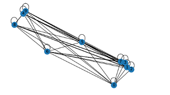

This code creates a graph object using the adjacency matrix, and then uses the NetworkX library’s draw function to visualize the graph. The with_labels=True argument tells the function to display the labels of the nodes. Finally, the plt.show() function is used to display the graph in a new window.

Alternatively, you can also visualize the node representations after training the GCN model using t-SNE or PCA:

from sklearn.manifold import TSNE

# Extract the learned node representations
node_representations = model(features, adjacency_matrix)

# Visualize the representations with t-SNE
tsne = TSNE(n_components=2)
node_representations_2d = tsne.fit_transform(node_representations.detach().numpy())

# Plot the 2D representations
plt.scatter(node_representations_2d[:, 0], node_representations_2d[:, 1])
plt.show()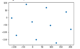

This code uses t-SNE to reduce the dimensionality of the node representations to 2, and then plots the 2D representations using a scatter plot.

It’s important to note that this is a simple example and in real-world scenarios, you may need to use more advanced techniques to visualize your data and models.

#Artificial Intelligence
#Machine Learning
#Data Science
#Neural Networks
#Beginner