The Naïve Bayes algorithm is one of the fundamental things to study when studying statistics of artificial intelligence. Here I’m going to explain naive Bayes.

It is very basic algorithm, yet one of most usefulusefull untill now.

Probability vs likelihood.

Generally, in machine learning, we know that past incidents (data points) are widely used to predict the future. It is not only mattering what happened in the past but also how probable it will be replicated in the future, known as the likelihood of an event occurring in a random space.

Let us take a simple example:
Suppose I have an unbiased 500 yen coin. When I flipped the coin, I can expect it will be the value side (tail). There is a 50% of possibility that my expectation comes true. (There are two possible outcomes, head and tail. Portability is calculated by (expected outcome/total no. of outcomes)
Now let us move a bit deep by operating two experiments at the same time. This time we are additionally rolling a dice. What is the probability of getting head by coin and getting 3 from dice?

The answer can be calculated as below;
P(Head & 3) = P(Head) * P(3) = 1/2 * 1/6 = 1/12

The term for the above example is called joint probability. Other than joint probability, there are two more two types, conditional probability and marginal probability.
1. Joint probability (probability of the coin landing on heads AND the dice landing on 3)
2. conditional probability (probability of heads GIVEN THAT the dice lands on 3)
3. marginal probability (probability of JUST the coin or JUST the dice)

The Bayes’ Theorem

It declares, for two events A & B, if we know the conditional probability of B given A and B’s probability, then it is possible to calculate the probability of B given A.

Let us move to a simple example to explain the Bayes rule.

Suppose that I have 30 BLUE objects and 60 RED objects. So there twice as many RED objects as BLUE. If I place a new object, it can be a RED since it is twice likely to happen rather than BLUE. This concept is called prior probability in Bayesian analysis.

Total objects = 90 (BLUE=30 + RED=60)
Prior probability of RED = Number of RED objects / total objects = 60/90
Prior probability of BLUE = Number of BLUE objects / total objects = 30/90

We finished calculating the prior probabilities. Now let us think that the new object is placed. Previously objects are well clustered. So we can assume that the new color of the new object can decide by the number of previous objects around the newly placed one.
If there are many BLUE objects, it can be BLUE, or If there are many REDS, it can be RED. To measure this likelihood, we form a circle around the new object which contains a number (to be determined a priori) of points regardless of their class names. Then we count the number of points in the circle fitting to each class name.

From hereafter, let us take the new object as X.
From the above drawing, we can see that the likelihood (possibility) of a X given RED is smaller than the likelihood of a X given BLUE since the circle contains the 1 RED and 3 BLUE objects.
In the previous section, the prior probabilities imply that X can relate to the RED since there are twice RED objects than the BLUE objects. However, we can see that likelihood contradicts the above. X can be BLUE since there are more BLUE than the RED around the X. We can calculate the posterior portability by multiplying by prior probability and likelihood.

Posterior Probability of RED=Prior Probability of RED ×Likelihood of RED =60/90×1/60

Posterior Probability of BLUE=Prior Probability of BLUE ×Likelihood of BLUE =30/90×3/30

By analyzing the calculation results, we can classify the new objects that belong to the BLUE since the Posterior Probability of BLUE is larger than the Posterior Probability of RED.

Example

In this example, you can use the dummy dataset with three columns: weather, temperature, and play. The first two are features(weather, temperature) and the other is the label.

# Assigning features and label variables
weather=['Sunny','Sunny','Overcast','Rainy','Rainy','Rainy','Overcast','Sunny','Sunny',
'Rainy','Sunny','Overcast','Overcast','Rainy']
temp=['Hot','Hot','Hot','Mild','Cool','Cool','Cool','Mild','Cool','Mild','Mild','Mild','Hot','Mild']

play=['No','No','Yes','Yes','Yes','No','Yes','No','Yes','Yes','Yes','Yes','Yes','No']

Encoding Features

First, you need to convert these string labels into numbers. for example: ‘Overcast’, ‘Rainy’, ‘Sunny’ as 0, 1, 2. This is known as label encoding. Scikit-learn provides LabelEncoder library for encoding labels with a value between 0 and one less than the number of discrete classes.

# Import LabelEncoder
from sklearn import preprocessing
#creating labelEncoder
le = preprocessing.LabelEncoder()
# Converting string labels into numbers.
wheather_encoded=le.fit_transform(wheather)
print wheather_encoded
#output ---> [2 2 0 1 1 1 0 2 2 1 2 0 0 1]

Similarly, you can also encode temp and play columns.

# Converting string labels into numbers
temp_encoded=le.fit_transform(temp)
label=le.fit_transform(play)
print "Temp:",temp_encoded

print "Play:",labelTemp: [1 1 1 2 0 0 0 2 0 2 2 2 1 2]
Play: [0 0 1 1 1 0 1 0 1 1 1 1 1 0]

Now combine both the features (weather and temp) in a single variable (list of tuples).

#Combinig weather and temp into single listof tuples
features=zip(weather_encoded,temp_encoded)
print features[(2, 1), (2, 1), (0, 1), (1, 2), (1, 0), (1, 0), (0, 0), (2, 2), (2, 0), (1, 2), (2, 2), (0, 2), (0, 1), (1, 2)]

Generating Model

Generate a model using naive bayes classifier in the following steps:

• Create naive bayes classifier
• Fit the dataset on classifier
• Perform prediction

#Import Gaussian Naive Bayes model
from sklearn.naive_bayes import GaussianNB

#Create a Gaussian Classifier
model = GaussianNB()

# Train the model using the training sets
model.fit(features,label)

#Predict Output
predicted= model.predict([[0,2]]) # 0:Overcast, 2:Mild
print "Predicted Value:", predicted

Predicted Value: [1]

Here, 1 indicates that players can ‘play’.

Naive Bayes with Multiple Labels

Till now you have learned Naive Bayes classification with binary labels. Now you will learn about multiple class classification in Naive Bayes. Which is known as multinomial Naive Bayes classification. For example, if you want to classify a news article about technology, entertainment, politics, or sports.

In model building part, you can use wine dataset which is a very famous multi-class classification problem. “This dataset is the result of a chemical analysis of wines grown in the same region in Italy but derived from three different cultivars.” (UC Irvine)

Dataset comprises of 13 features (alcohol, malic_acid, ash, alcalinity_of_ash, magnesium, total_phenols, flavanoids, nonflavanoid_phenols, proanthocyanins, color_intensity, hue, od280/od315_of_diluted_wines, proline) and type of wine cultivar. This data has three type of wine Class_0, Class_1, and Class_3. Here you can build a model to classify the type of wine.

The dataset is available in the scikit-learn library.

Loading Data

Let’s first load the required wine dataset from scikit-learn datasets.

#Import scikit-learn dataset library
from sklearn import datasets

#Load dataset
wine = datasets.load_wine()

Exploring Data

You can print the target and feature names, to make sure you have the right dataset, as such:

# print the names of the 13 features
print "Features: ", wine.feature_names

# print the label type of wine(class_0, class_1, class_2)
print "Labels: ", wine.target_names

Features: ['alcohol', 'malic_acid', 'ash', 'alcalinity_of_ash', 'magnesium', 'total_phenols', 'flavanoids', 'nonflavanoid_phenols', 'proanthocyanins', 'color_intensity', 'hue', 'od280/od315_of_diluted_wines', 'proline']
Labels: ['class_0' 'class_1' 'class_2']

It’s a good idea to always explore your data a bit, so you know what you’re working with. Here, you can see the first five rows of the dataset are printed, as well as the target variable for the whole dataset.

Splitting Data

First, you separate the columns into dependent and independent variables(or features and label). Then you split those variables into train and test set.

# Import train_test_split function
from sklearn.cross_validation import train_test_split

# Split dataset into training set and test set
X_train, X_test, y_train, y_test = train_test_split(wine.data, wine.target, test_size=0.3,random_state=109) # 70% training and 30% test

Model Generation

After splitting, you will generate a random forest model on the training set and perform prediction on test set features.

#Import Gaussian Naive Bayes model
from sklearn.naive_bayes import GaussianNB

#Create a Gaussian Classifier
gnb = GaussianNB()

#Train the model using the training sets
gnb.fit(X_train, y_train)

#Predict the response for test dataset
y_pred = gnb.predict(X_test)

Evaluating Model

After model generation, check the accuracy using actual and predicted values.

#Import scikit-learn metrics module for accuracy calculation
from sklearn import metrics

# Model Accuracy, how often is the classifier correct?
print("Accuracy:",metrics.accuracy_score(y_test, y_pred))

('Accuracy:', 0.90740740740740744)

Zero Probability Problem

Suppose there is no tuple for a risky loan in the dataset, in this scenario, the posterior probability will be zero, and the model is unable to make a prediction. This problem is known as Zero Probability because the occurrence of the particular class is zero.

The solution for such an issue is the Laplacian correction or Laplace Transformation. Laplacian correction is one of the smoothing techniques. Here, you can assume that the dataset is large enough that adding one row of each class will not make a difference in the estimated probability. This will overcome the issue of probability values to zero.

For Example: Suppose that for the class loan risky, there are 1000 training tuples in the database. In this database, income column has 0 tuples for low income, 990 tuples for medium income, and 10 tuples for high income. The probabilities of these events, without the Laplacian correction, are 0, 0.990 (from 990/1000), and 0.010 (from 10/1000)

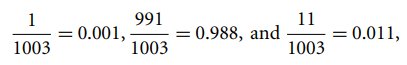
Now, apply Laplacian correction on the given dataset. Let’s add 1 more tuple for each income-value pair. The probabilities of these events:

What are the Pros and Cons of Naive Bayes?

Pros:

• It is easy and fast to predict class of test data set. It also perform well in multi class prediction
• When assumption of independence holds, a Naive Bayes classifier performs better compare to other models like logistic regression and you need less training data.
• It perform well in case of categorical input variables compared to numerical variable(s). For numerical variable, normal distribution is assumed (bell curve, which is a strong assumption).

Cons:

• If categorical variable has a category (in test data set), which was not observed in training data set, then model will assign a 0 (zero) probability and will be unable to make a prediction. This is often known as “Zero Frequency”. To solve this, we can use the smoothing technique. One of the simplest smoothing techniques is called Laplace estimation.
• On the other side naive Bayes is also known as a bad estimator, so the probability outputs from predict_proba are not to be taken too seriously.
• Another limitation of Naive Bayes is the assumption of independent predictors. In real life, it is almost impossible that we get a set of predictors which are completely independent.

Applications of Naive Bayes Algorithms

• Real time Prediction: Naive Bayes is an eager learning classifier and it is sure fast. Thus, it could be used for making predictions in real time.
• Multi class Prediction: This algorithm is also well known for multi class prediction feature. Here we can predict the probability of multiple classes of target variable.
• Text classification/ Spam Filtering/ Sentiment Analysis: Naive Bayes classifiers mostly used in text classification (due to better result in multi class problems and independence rule) have higher success rate as compared to other algorithms. As a result, it is widely used in Spam filtering (identify spam e-mail) and Sentiment Analysis (in social media analysis, to identify positive and negative customer sentiments)
• Recommendation System: Naive Bayes Classifier and Collaborative Filtering together builds a Recommendation System that uses machine learning and data mining techniques to filter unseen information and predict whether a user would like a given resource or not

Thanks for Reading such long Article. I have only tried to cover the basics. If you are interested do messeage me I can post some interesting projects where still i prefer Naive bayer over the Strong Neural Network models.

— — — — — — — — — — — — — — — — — — — — — — — — — — — — — — — —

#Naive Bayes

#Artificial Intelligence

#Machine Learning

#Towards Data Science

#Beginners Guide