GANs Architecture in Detail!(Part-3)

The GAN model works by having the generator try to create realistic images that the discriminator cannot distinguish from real images. The discriminator, on the other hand, tries to accurately classify the images as real or fake. The two models are trained simultaneously, with the generator trying to improve its image generation capabilities and the discriminator trying to improve its ability to distinguish real from fake images.

During training, the generator and discriminator are fed a combination of real and fake images, and the output of each model is used to update the weights of the other model. The generator’s goal is to create images that are indistinguishable from real images, while the discriminator’s goal is to accurately classify the images as real or fake.

One of the challenges of training GANs is balancing the performance of the generator and discriminator. If the generator becomes too good at creating realistic images, the discriminator may not be able to keep up and will not be able to provide useful feedback to the generator. On the other hand, if the discriminator becomes too good at distinguishing fake images, the generator may not be able to improve and the GAN will not be able to generate high-quality images.

The concept of adversarial learning, in which two models compete with each other to improve their performance, has the potential to lead to significant breakthroughs in machine learning. By exploring this framework further, researchers may be able to develop more advanced machine learning systems that are capable of performing tasks that are currently beyond the reach of traditional machine learning methods.

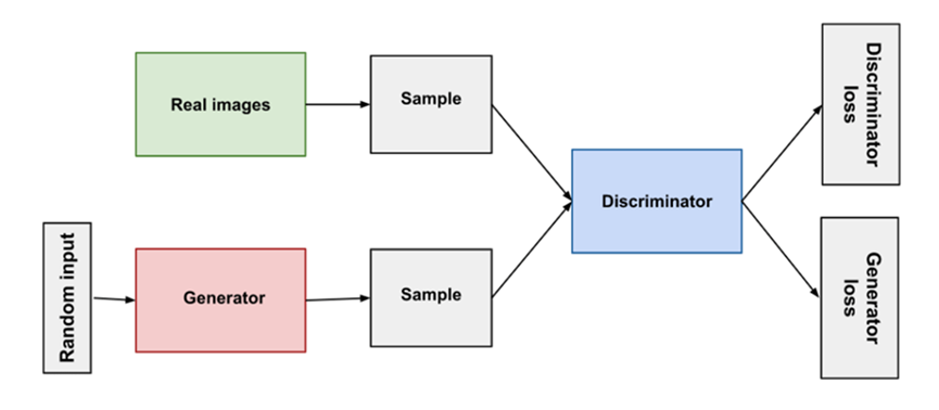
image source — developers.google.com

DNNs

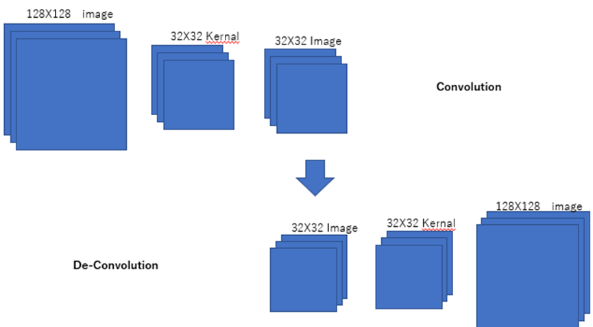
The deconvolutional neural network (DNN) is a key component of the GAN, responsible for generating images from random input values (noise). Deconvolutional neural networks, also known as transposed convolutional neural networks or deconvs, use layers similar to those found in convolutional neural networks (CNNs), but in reverse order, to upsample the input image and produce an output image that is larger than the original.

One of the challenges of deconvolution is that it is more difficult to make an image larger without introducing blurriness or loss of detail. This problem is addressed with the transposed convolution (deconvolution) operation, which involves applying a kernel to the upsampled image and producing an output image that is larger than the original image.

To understand deconvolution or transposed convolution , it is helpful to first understand the concept of convolution. A convolution is a mathematical operation that takes two input functions (the “input” and “kernel” functions) and produces an output function. In the context of image processing, the input function is often an image and the kernel is a small matrix of weights. The convolution operation involves applying the kernel to each position in the image, multiplying the values in the kernel by the corresponding values in the image, and summing the results. The output of the convolution is a new image, which is often smaller than the original image.

The transposed convolution (also known as a deconvolution) is essentially the inverse operation of a convolution. It involves upsampling the input image, applying the kernel to the upsampled image, and producing an output image that is larger than the original image. Deconvolution is used in GANs to generate new images from random noise.

In order to understand how deconvolution works, it is helpful to understand the concept of padding. Padding is the process of adding extra pixels around the edges of an image to preserve the spatial relationships between the pixels in the original image. For example, consider an image with a single pixel. If we apply a convolution with a kernel that has a 3×3 matrix of weights, the output image will have a single pixel as well. However, if we pad the original image with a border of zeros, the output image will have a 3×3 matrix of pixels, with the center pixel being the result of the convolution operation.

In the case of a deconvolution, the padding is removed from the output image, resulting in an image that is larger than the original image. The kernel is applied to the upsampled image, and the resulting image is the output of the deconvolution. This process can be repeated multiple times to generate larger and larger images.

created by Author

def Generator():
    model = tf.keras.Sequential()
    model.add(layers.Dense(128*128*3, use_bias=False, input_shape=(latent_dim,)))
    model.add(layers.Reshape((128,128,3)))
    # downsampling
    model.add(tf.keras.layers.Conv2D(128,4, strides=1, padding='same',kernel_initializer='he_normal', use_bias=False))
    model.add(tf.keras.layers.Conv2D(128,4, strides=2, padding='same',kernel_initializer='he_normal', use_bias=False))
    model.add(tf.keras.layers.BatchNormalization())
    model.add(tf.keras.layers.LeakyReLU())
    model.add(tf.keras.layers.Conv2D(256,4, strides=1, padding='same',kernel_initializer='he_normal', use_bias=False))
    model.add(tf.keras.layers.Conv2D(256,4, strides=2, padding='same',kernel_initializer='he_normal', use_bias=False))
    model.add(tf.keras.layers.BatchNormalization())
    model.add(tf.keras.layers.LeakyReLU())
    model.add(tf.keras.layers.Conv2DTranspose(512, 4, strides=1,padding='same',kernel_initializer='he_normal',use_bias=False))
    model.add(tf.keras.layers.Conv2D(512,4, strides=2, padding='same',kernel_initializer='he_normal', use_bias=False))
    
    model.add(tf.keras.layers.LeakyReLU())
    #upsampling
    model.add(tf.keras.layers.Conv2DTranspose(512, 4, strides=1,padding='same',kernel_initializer='he_normal',use_bias=False))
    model.add(tf.keras.layers.Conv2DTranspose(512, 4, strides=2,padding='same',kernel_initializer='he_normal',use_bias=False))
    model.add(tf.keras.layers.BatchNormalization())
    model.add(tf.keras.layers.LeakyReLU())
    model.add(tf.keras.layers.Conv2DTranspose(256, 4, strides=1,padding='same',kernel_initializer='he_normal',use_bias=False))
    model.add(tf.keras.layers.Conv2DTranspose(256, 4, strides=2,padding='same',kernel_initializer='he_normal',use_bias=False))
    model.add(tf.keras.layers.BatchNormalization())
    
    model.add(tf.keras.layers.Conv2DTranspose(128, 4, strides=2,padding='same',kernel_initializer='he_normal',use_bias=False))
    model.add(tf.keras.layers.Conv2DTranspose(128, 4, strides=1,padding='same',kernel_initializer='he_normal',use_bias=False))
    model.add(tf.keras.layers.BatchNormalization())
    model.add(tf.keras.layers.Conv2DTranspose(3,4,strides = 1, padding = 'same',activation = 'tanh'))
    return model

def Discriminator():
    model = tf.keras.models.Sequential()
    model.add(tf.keras.layers.Input((SIZE, SIZE, 3)))
    model.add(tf.keras.layers.Conv2D(128,4, strides=2, padding='same',kernel_initializer='he_normal', use_bias=False))
    model.add(tf.keras.layers.BatchNormalization())
    model.add(tf.keras.layers.LeakyReLU())
    model.add(tf.keras.layers.Conv2D(128,4, strides=2, padding='same',kernel_initializer='he_normal', use_bias=False))
    model.add(tf.keras.layers.BatchNormalization())
    model.add(tf.keras.layers.LeakyReLU())
    model.add(tf.keras.layers.Conv2D(256,4, strides=2, padding='same',kernel_initializer='he_normal', use_bias=False))
    model.add(tf.keras.layers.BatchNormalization())
    model.add(tf.keras.layers.LeakyReLU())
    model.add(tf.keras.layers.Conv2D(256,4, strides=2, padding='same',kernel_initializer='he_normal', use_bias=False))
    model.add(tf.keras.layers.BatchNormalization())
    model.add(tf.keras.layers.LeakyReLU())
    model.add(tf.keras.layers.Conv2D(512,4, strides=2, padding='same',kernel_initializer='he_normal', use_bias=False))
    model.add(tf.keras.layers.LeakyReLU())
    model.add(tf.keras.layers.Flatten())
    model.add(tf.keras.layers.Dense(1,activation = 'sigmoid'))
    return model

Challenges of training GANs

There are several approaches to address the challenges of training GANs, such as using different training algorithms or architectural designs for the generator and discriminator, using different types of loss functions, or using techniques such as feature matching or mini-batch discrimination to stabilize the training process.

One popular training algorithm for GANs is the Wasserstein GAN (WGAN), which uses the Wasserstein distance (also known as the Earth Mover’s distance) as the loss function for the discriminator. The Wasserstein distance measures the amount of work required to transform one distribution of data into another, and has been shown to be a more stable loss function for GAN training compared to the commonly used cross-entropy loss.

Another approach to improving the stability of GAN training is to use techniques such as feature matching, which involves training the generator to match the statistics of the real data rather than trying to fool the discriminator. This can help to avoid the problem of mode collapse, as the generator is encouraged to produce a diverse range of images rather than focusing on a single mode.

Summary

In summary, GANs are a powerful machine learning framework that are capable of generating realistic images and videos. However, training GANs can be challenging due to problems such as the discriminator overpowering the generator or mode collapse. There are various approaches to address these challenges, including using different training algorithms and techniques, and adjusting the architecture and training of the generator and discriminator.

— — — — — — — — — — — — — — — — — — — — — — — — — — — — — — — —

If you like reading stories like this and want to support my writing, Please consider to follow me. As a medium member, you have unlimited access to thousands of Python guides and Data science articles.

#Generative Adversarial

#Artificial Intelligence

#Machine Learning

#Deep Learning

#Towards Data Science